Profit maximization
In economics, profit maximization is the (short run) process by which a firm determines the price and output level that returns the greatest profit. There are several approaches to this problem. The total revenue–total cost method relies on the fact that profit equals revenue minus cost, and the marginal revenue–marginal cost method is based on the fact that total profit in a perfectly competitive market reaches its maximum point where marginal revenue equals marginal cost.
Contents |
Basic definitions
Any costs incurred by a firm may be classed into two groups: fixed costs and variable costs. Fixed costs are incurred by the business at any level of output, including zero output. These may include equipment maintenance, rent, wages, and general upkeep. Variable costs change with the level of output, increasing as more product is generated. Materials consumed during production often have the largest impact on this category. Fixed cost and variable cost, combined, equal total cost.
Revenue is the amount of money that a company receives from its normal business activities, usually from the sale of goods and services (as opposed to monies from security sales such as equity shares or debt issuances).
Marginal cost and revenue, depending on whether the calculus approach is taken or not, are defined as either the change in cost or revenue as each additional unit is produced, or the derivative of cost or revenue with respect to quantity output. It may also be defined as the addition to total cost or revenue as output increase by a single unit. For instance, taking the first definition, if it costs a firm 400 USD to produce 5 units and 480 USD to produce 6, the marginal cost of the sixth unit is approximately 80 dollars, although this is more accurately stated as the marginal cost of the 5.5th unit due to linear interpolation. Calculus is capable of providing more accurate answers if regression equations can be provided.
Total revenue - total cost method
To obtain the profit maximising output quantity, we start by recognizing that profit is equal to total revenue (TR) minus total cost (TC). Given a table of costs and revenues at each quantity, we can either compute equations or plot the data directly on a graph. Finding the profit-maximizing output is as simple as finding the output at which profit reaches its maximum. That is represented by output Q in the diagram.
There are two graphical ways of determining that Q is optimal. First, the profit curve is at its maximum at this point (A). Secondly, at the point (B) the tangent on the total cost curve (TC) is parallel to the total revenue curve (TR), meaning that the surplus of revenue net of costs (B,C) is at its greatest. Because total revenue minus total costs is equal to profit, the line segment C,B is equal in length to the line segment A,Q.
Computing the price at which to sell the product requires knowledge of the firm's demand curve. The price at which quantity demanded equals profit-maximizing output is the optimum price to sell the product.
Marginal revenue-marginal cost method
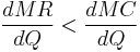
An alternative argument says that for each unit sold, marginal profit (Mπ) equals marginal revenue (MR) minus marginal cost (MC). Then, if marginal revenue is greater than marginal cost, marginal profit is positive, and if marginal revenue is less than marginal cost, marginal profit is negative. When marginal revenue equals marginal cost, marginal profit is zero.[1] Since total profit increases when marginal profit is positive and total profit decreases when marginal profit is negative, it must reach a maximum where marginal profit is zero - or where marginal cost equals marginal revenue. If there are two points where this occurs, maximum profit is achieved where the producer has collected positive profit up until the intersection of MR and MC (where zero profit is collected), but would not continue to after, as opposed to vice versa, which represents a profit minimum.[1] In calculus terms, the correct intersection of MC and MR will occur when:[1]
The intersection of MR and MC is shown in the next diagram as point A. If the industry is perfectly competitive (as is assumed in the diagram), the firm faces a demand curve (D) that is identical to its Marginal revenue curve (MR), and this is a horizontal line at a price determined by industry supply and demand. Average total costs are represented by curve ATC. Total economic profit are represented by area P,A,B,C. The optimum quantity (Q) is the same as the optimum quantity (Q) in the first diagram.
If the firm is operating in a non-competitive market, minor changes would have to be made to the diagrams. For example, the Marginal Revenue would have a negative gradient, due to the overall market demand curve. In a non-competitive environment, more complicated profit maximization solutions involve the use of game theory.
Maximizing revenue method
In some cases a firm's demand and cost conditions are such that marginal profits are greater than zero for all levels of production.[2] In this case the Mπ = 0 rule has to be modified and the firm should maximize revenue.[2] In other words the profit maximizing quantity and price can be determined by setting marginal revenue equal to zero. Marginal revenue equals zero when the Total revenue curve has reached its maximum value. An example would be a scheduled airline flight. The marginal costs of flying the route are negligible. The airline would maximize profits by filling all the seats. The airline would determine the  conditions by maximizing revenues.
Changes in total costs and profit maximization
A firm maximizes profit by operating where marginal revenue equal marginal costs. A change in fixed costs has no effect on the profit maximizing output or price.[3] The firm merely treats short term fixed costs as sunk costs and continues to operate as before.[4] This can be confirmed graphically. Using the diagram illustrating the total cost total revenue method the firm maximizes profits at the point where the slope of the total cost line and total revenue line are equal.[2] A change in total cost would cause the total cost curve to shift up by the amount of the change.[2] There would be no effect on the total revenue curve or the shape of the total cost curve. Consequently, the profit maximizing point would remain the same. This point can also be illustrated using the diagram for the marginal revenue marginal cost method. A change in fixed cost would have no effect on the position or shape of these curves.[2]
Markup pricing
In addition to using methods to determine a firm's optimal level of output, a firm can also set price to maximize profit. Profit maximization requires that a firm produce where marginal revenue equals marginal costs. Firm managers are unlikely to have complete information concerning their marginal revenue function or their marginal costs. [5] Fortunately the profit maximization conditions can be expressed in a "more easily applicable" form or rule of thumb.[5] The first step is to rewrite the expression for marginal revenue as MR = ∆TR/∆Q =(P∆Q+Q∆P)/∆Q=P+Q∆P/∆Q.[5] The marginal revenue from an "incremental unit of quantity" has two parts: first, the revenue the firm gains from selling the additional units or P∆Q. The additional units are called the marginal units.[6] Producing one extra unit and selling it a P brings in revenue of P. Second, "the revenue the firm loses on the units it could have sold at the higher price."[6] These lost units are called the infra-marginal units.[6] That is selling the extra unit results in a small drop in price which reduces the revenue for all units sold. Q(∆P/∆Q) Thus MR = P + Q(∆P/∆Q) = P +P (Q/P)((∆P/∆Q) = P + P(1/(PED) Then setting MR = MC MC = P + P(1/(PED) P - MC/P = - 1/PED P = MC/1 + (1/PED). The optimal markup rule is:
- (P - MC)/P = 1/ -Ep
- or
- P = (Ep/(1 + Ep)) MC[7]
Where MC equals marginal costs and Ep equals price elasticity of demand for the firm (not the market PED).[8] Ep is a negative number. Therefore, -Ep is a positive number.
In English the rule is that the size of the markup is inversely related to the price elasticity of demand for a good.[7]
The optimal markup rule also implies that a non-competitive firm will produce on the elastic region of its market demand curve. Marginal costs is positive. The term 1/ -Ep would be positive only if the PED is between -1 and -∝ that is if demand is elastic.[9]
MPL, MRPL and profit maximization
The general rule is that firm maximizes profit by producing that quantity of output where marginal revenue equals marginal costs. The profit maximization issue can also be approached from the input side. That is, what is the profit maximizing usage of the variable input? [10] To maximize profits the firm should increase usage "up to the point where the input's marginal revenue product equals its marginal costs".[11] So mathematically the profit maximizing rule is MRPL = MCL The marginal revenue product is the change in total revenue per unit change in the variable input assume labor. That is MRPL = ∆TR/∆L. MRPL is the product of marginal revenue and the marginal product of labor or MRPL = MR x MPL.
See also
- Business organization
- Corporation
- Market forms
- Microeconomics
- Pricing
- Production, costs, and pricing
- Rational choice theory
- Supply and demand
- Marginal revenue
- Total revenue
Notes
- ^ a b c Lipsey (1975). pp. 245-47.
- ^ a b c d e Samuelson, W and Marks, S (2003). p. 47.
- ^ Samuelson, W and Marks, S (2003). p. 52.
- ^ Landsburg, S (2002).
- ^ a b c Pindyck, R and Rubinfeld, D (2001) p. 333.
- ^ a b c Besanko, D. and Beautigam, R, (2001) p. 408.
- ^ a b Samuelson, W and Marks, S (2003). p. 103-05.
- ^ Pindyck, R and Rubinfeld, D (2001) p. 341.
- ^ Besanko and Braeutigam (2005) p. 419.
- ^ Samuelson, W and Marks, S (2003). p. 230.
- ^ Samuelson, W and Marks, S (2003). p. 23.
References
- Landsburg, S (2002). Price Theory and Applications (fifth ed.). South-Western.
- Lipsey, Richard G. (1975). An introduction to positive economics (fourth ed.). Weidenfeld and Nicolson. pp. 214–7. ISBN 0297768999.
- Samuelson, W; Marks, S (2003). Managerial Economics (fourth ed.). Wiley.
External links
- Profit Maximization in Perfect Competition by Fiona Maclachlan, Wolfram Demonstrations Project.